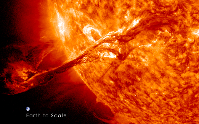
On August 31, 2012 a long filament of solar material that had been hovering in the sun’s atmosphere, the corona, erupted out into space at 4:36 p.m. EDT. The coronal mass ejection, or CME, traveled at over 900 miles per second. The CME did not travel directly toward Earth, but did connect with Earth’s magnetic environment, or magnetosphere, causing aurora to appear on the night of Monday, September 3. The image above includes an image of Earth to show the size of the CME compared to the size of Earth. NASA Goddard Spaceflight Center

Thursday, May 2nd, 2013, a coronal mass ejection (CME) hurled nearly one billion tons of charged particles from the sun’s corona at an outward velocity of one million miles per hour – 270 miles per second.

In less than a half hour, 2,700 virtual Empire State Buildings, 340,000 tons apiece – give or take a few gorillas – erupted from an active region of the Sun’s surface called AR1748, a northern latitude sunspot. AR1748 had just become visible on the western limb of the Sun’s surface when it ejected this mass, so the vast bulk of it hurled outward, not toward us in Libra, but more or less toward Cancer, at right-angles to us. In practical terms, it shot wide of its mark. Still an impressive shot. The CME had been triggered by an M class solar flare, the second largest in a five step scheme (An, Bn, Cn, Mn, Xn; for n a relative magnitude). It had been the largest coronal mass ejection observed thus far in 2013.

And it was still early in the day for AR1748.

Beginning an approximately month-long trek across the Sun’s face, AR1748 remained quiescent over the next ten days until Mother’s Day, May 12, when it emitted an X1.7 class solar flare. Fourteen hours later AR1748 emitted an X2.8 class solar flare, almost twice as powerful as the Mother’s Day flare and over four times as powerful as the M class flare at the top of the month. Eight hours later, early Tuesday morning, AR1748 flared for a third time, an X3.2 class event, a fourth time on May 15, an X1.0 event, a fifth time on Thursday, May 16th, a small C4.0 solar flare, and, as of this writing, a  sixth flare on the 17th, an M3.2 event. The X2.8 flare also triggered a CME, which missed the Earth, but the whiz of the round was louder in our ears than the May 2nd miss. It disrupted high frequency radio communications in a number of areas. The fourth X1.0 event on May 15 pitched out a CME that brushed the Earth’s magnetosphere on May 17th. Canadian and Alaskan readers might have seen some pretty Northern Lights that night and the atmosphere experienced a mild geomagnetic storm, arising from charged particles from the CME interacting with the magnetosphere.

We expect that you get the picture: The Sun, a stately rotating turret, is festooned with cannon – sunspots – which, at unpredictable intervals, fire off coronal mass ejections of varying sizes. Most the time, nearly all of the time, we’re nowhere near the firing line. On occasion, we’re dead center in the cross hairs, the times when we really hope the damn things won’t shoot off. To confound matters a little, coronal mass ejections sometimes reel off the Sun without any sunspot being near. Conversely, sunspots sometimes emit solar flares without CME events. In any case, the effect is one of being in a celestial shooting gallery. However, even if we were free from our gravitational bounds, we would not move from the bull’s eye, because though the sun shoots at us, it also gives us life.

Around Saturday, May 18th , we slid into the cross-hairs of AR1748 and remained there until early this week, when AR1748 rotated off the eastern rim. Other sunspots are heaving into view, however, so with AR1748 exiting stage right, new ones, perhaps very active ones, are entering stage left. And so it goes. AR1748 was accompanied by as many as ten sunspots transiting the solar face, and, among that lot, was the most trigger happy. Welcome to Solar Cycle 24, whose peak, the height of an eleven year sunspot cycle, is now well nigh upon us.

So what happens if we get shot?

It could be a lot. For a big enough flare, a total radio blackout across the high frequency radio spectrum could last upward to a day or two. Shortwave radio depends on the ionosphere to bounce signals great distances, and the disruption of the ionosphere affects this phenomenon. If the solar flare contains hard X-rays, then a failure of most orbiting electronics can take place, giving rise to a bevy of outages for many industries which depend on satellites: GPS, telecommunications and other core services. But the grand-daddy catastrophe that keeps most planners up at night is the potential collapse of electrical power grids – especially the largest, North American power grid – and the attendant disasters which would inevitably spin off from such a collapse.

Transformers, represented here by overlapping rings, are ubiquitous in the power grid. Generator Step Up (GSU) transformers may raise generator voltage levels five to thirty times for long distance transmission (blue lines). Substation transformers feed distribution grids (green lines); the currents of these grids are matched to the needs of end users through hundreds of delivery transformers. With wires spanning hundreds of miles, transmission grids are very susceptible to geomagnetic induced currents.

This illustration  depicts an extremely basic power grid. It is missing a ton of stuff, but the components essential to power distribution – and which are also sensitive to a coronal mass ejection – are in place.
The two key parts of this distribution system are (1) alternating current generators, which provide energy, and (2) transformers, which inductively couple circuits into continent-spanning distribution systems. The Induction Law is the essential relation which makes transformers in power distribution systems effective. It bases a transformer’s ability to step up or step down voltages to the ratio of turns in its primary and secondary coils, across which inductive coupling takes place.

Transformers at generating stations step up voltages to as high as 765 kilovolts for transmission. Losses arise from current flow and at very high voltages correspondingly little current is required to convey a given parcel of energy. But since extremely high voltages are very hazardous, transformers in distribution farms step down voltages to one kilovolt for regional electrical lines. Small transformers, roughly the size of kitchen refrigerators, feed 120 and 220 volt domestic lines – at least in North America. Other voltages apply in other parts of the world.

Transformers need alternating current because inductive coupling only works when magnetic fields are constantly changing direction. It is the rate of change of magnetic flux around a primary coil over time that induces electric current in a secondary coil. Steady, unvarying, direct current builds steady, unvarying magnetic fields and, except at power-on or power-off, these steady magnetic fields do not couple primary and secondary coils. It was this factor that gave primacy to alternating over direct current during the evolution the country’s power grids at the turn of the Twentieth Century.

No matter what the operating voltage is, a transformer’s operating sweet spot centers on zero volts. Even on 765 kilovolt lines each positive swing is counterbalanced by a negative swing, with the whole ensemble averaging zero volts over time. With a transformer’s magnetic field building first to one polarity, then to the other, its iron core does not saturate.

All the physics of the power distribution system are very well understood. Where it gets tricky is when the highly charged particles of a coronal mass ejection interact with the magnetosphere surrounding our planet. Then some pretty outlandish physics gets into play. We’ll look at some of that in Part Three.

Previous: Celestial Shooting Gallery, Part One: The Day We Lost Quebec

Next: Celestial Shooting Gallery, Part Three: When a CME Hits the Atmosphere