1. The State of Gerrymandering in these United States
In our last post, we wrote about how to compute the Gerrymander Index of shapes, including Congressional districts. Since then we’ve fetched the U. S. Census Bureau tl_2014_us_cd114 Esri shapefile data set of the 435 Congressional Districts for the current 114th Congress, which includes the nine non-voting districts that send delegates to Congress. If you are terminally curious, download the comma-separated value text file of our results, based on Census Bureau dataset. We’re not going to discuss all 444 maps; restricting our attention to the best and the worst, the state of gerrymandering in these United States, and how the States of California and Texas are gerrymandering these days.
Of the four hundred forty four records in tl_2014_us_cd114, the most gerrymandered district is North Carolina Congressional District 12, with a Gerrymander Index of 0.0291, this based on its cartographic boundary as defined in the Census Bureau shape file.
It is worth having a look at this district (Illustration 2). It includes sections of Winston-Salem, Greensboro and High Point in the north (The “Piedmont Triad”) then meanders south by south-west about eighty miles to Charlotte, where it cherry-picks communities within the I-485 beltway, excluding Marlboro to the south.
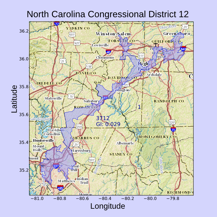
2. North Carolina Congressional District 12 for the 114th Congress
“Cherry picking” pretty much sums up how the district came about. Its current incarnation emerged after the 1990 census, when North Carolina gained its twelfth seat in the House of Representatives. At the time, Supreme Court decisions and Justice Department rulings enforcing Section 2 of the 1965 Voting Rights Act had called for North Carolina to redress under-representation of African-American minorities, the particular approach being left to the state. The North Carolina legislature. under Democratic control in 1992, responded by linking together minority (and also Democratic) districts in the four cities, with little regard to whether they were “compact” in a locale. It was, unabashedly, an exercise in packing, nominally in deference of the Voting Rights Act, but also fashioning a Democratic “safe seat” in the heart of a Republican stronghold. Since its inception, the 12th has consistently sent Democrats to the House.
This had not gone unnoticed. At the district’s inception, the Wall Street Journal called it “political pornography”. In somewhat more measured tones, Justice Sandra Day O’Connor wrote in her opinion of Shaw v. Reno:
“A reapportionment plan that includes in one district individuals who belong to the same race, but who are otherwise widely separated by geographical and political boundaries, and who may have little in common with one another but the color of their skin, bears an uncomfortable resemblance to political apartheid. It reinforces the perception that members of the same racial group–regardless of their age, education, economic status, or the community in which they live–think alike, share the same political interests, and will prefer the same candidates at the polls … By perpetuating such notions, a racial gerrymander may exacerbate the very patterns of racial bloc voting that majority-minority districting is sometimes said to counteract.”
The district lines were modified following the 2000 and 2010 Census, eliminating some of its more bizarre features, such as following highways for miles without including households on either side. The present configuration is marginally more “compact” but remains as one of the more gerrymandered districts in the nation.
North Carolina itself is one of the more gerrymandered states in the nation. The average Gerrymander Index of the state’s thirteen districts is 0.117, ranging from the 12th District’s 0.029 to the 8th District’s fairly respectable 0.223. It vies with West Virginia for top gerrymander honors, which comes in as a close secondi at 0.137. However, West Virginia is deep within Appalachia. People there live in the rift valleys that nestle between mountain ranges, and these influence the lay of roads, towns, counties and even the state itself, giving rise to elongated regions centered on northeast-southwest axes. This topography characterizes the western extreme of North Carolina as well, but the middle and eastern portions of the state, about eighty percent of its area, consists of the Piedmont region, occupying the middle third of the state, and the Atlantic coastal region, a little less than half of the eastern part of the state. The Piedmont is a region of foothills; the Atlantic coastal region is flat. Neither topology forces a particular shape to towns or counties.
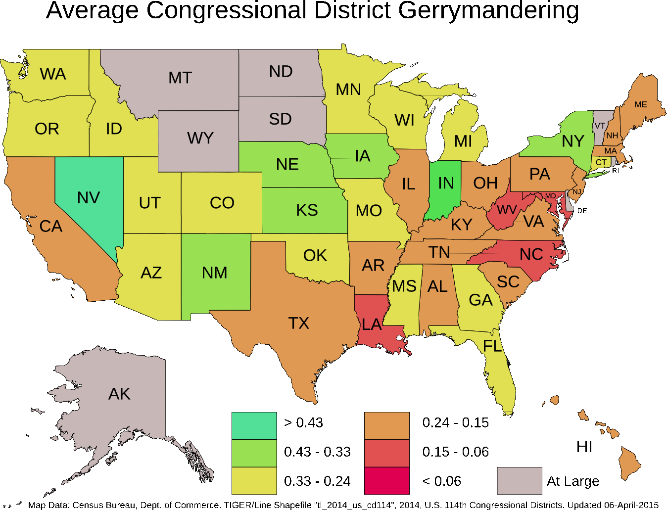
Nor is gerrymandering confined to North Carolina; indeed it seems a regional epidemic. We composed a map of state averages of gerrymandering (Illustration One) and found that the Mid-Atlantic region, east of the Mississippi, south of Pennsylvania and the Ohio River and north of the 35° parallel, has six states below the national gerrymander average of about 0.28. Delaware, the exception, has no Congressional Districts, formally sending one “Representative at large” to the House. Certainly the Appalachians contribute to this effect, but how much so is open to debate.

3. Indiana 1st Congressional District, around Gary and East Chicago, IN
Illustration 3: Indiana 1st Congressional District, around Gary and East Chicago, IN
At the other extreme, the least gerrymandered Congressional District appears to be Indiana 1st Congressional District, with a Gerrymander Index of 0.561. It is a district in a state where all districts except one exceed the national average, and the state average itself is 0.436.
Situated in the state’s northwest corner, encompassing Gary IN, its southern edge traces the Kankakee River and it has a tiny eastern panhandle along the Lake Michigan shoreline that encompasses the towns of Hesston and Smith ten miles further east from the county border that the district line otherwise follows – a whiff of gerrymandering, perhaps. Gary has been the District’s traditional core; 70% of the population live there. The seat has been Democratic since 1931 and the present Representative, Peter Visclosky, has held the seat since 1985. It seems like a pretty safe seat.
This certainly can raise eyebrows among political cynics, but the longevity of Democrats make sense. Gary is an old steel mill town, currently suffering Rust Belt economics. U. S. Steel founded the city in 1906 to support its Gary Works, nearly a hundred years on, still the city’s biggest employer, though that employment has dropped from a high of 30,000 to a current level of around 6,000. It is the home of many blue collar, unionized workers. The district, drawn compactly around Gary, simply, and unsurprisingly, reflects the politics of Gary. In a similar unsurprising vein, the other districts in the state reflect the political dispositions of rural, conservative agrarians with Republican leanings. With one exception, the districts have simple boundaries with high Gerrymander Indices. The Indiana 8th Congressional District, with a Gerrymander Index of 0.217, is the lowest in the state, but this low index does not seem due to high art. The Wabash River borders the district on the west and the Ohio on the south, both sinuous waterways, each with many cut-offs and switchbacks, meandering through prairie lands. Natural causes, not mischievous politics, seem to be at the root.
As a national phenomenon, gerrymandering seems more prevalent east of Longitude −94°, about the meridian of Kansas City. Most states west of this meridian have Congressional Districts at or above the national average Gerrymander Index of 0.28. These are square prairie states with square counties, square towns and square congressional districts, an unimaginative state of affairs, perhaps, but uncomplicated. The two exceptions are California and Texas, the states with the largest (California: 53) and second largest (Texas: 36) Congressional delegations. Both states have had controversial districting plans enacted since the start of the current century.
In 2008, California voters narrowly approved Proposition 11, transferring redistricting authority from the California State legislature to a fourteen member Citizen’s Redistricting Commission consisting of five Democrats, five Republicans and four from other political or “independent” alignments. Initially instituted for just state-level offices, California voters augmented the commission’s authority in 2010 with Proposition 20, transferring the responsibility for Congressional redistricting to the commission as well.
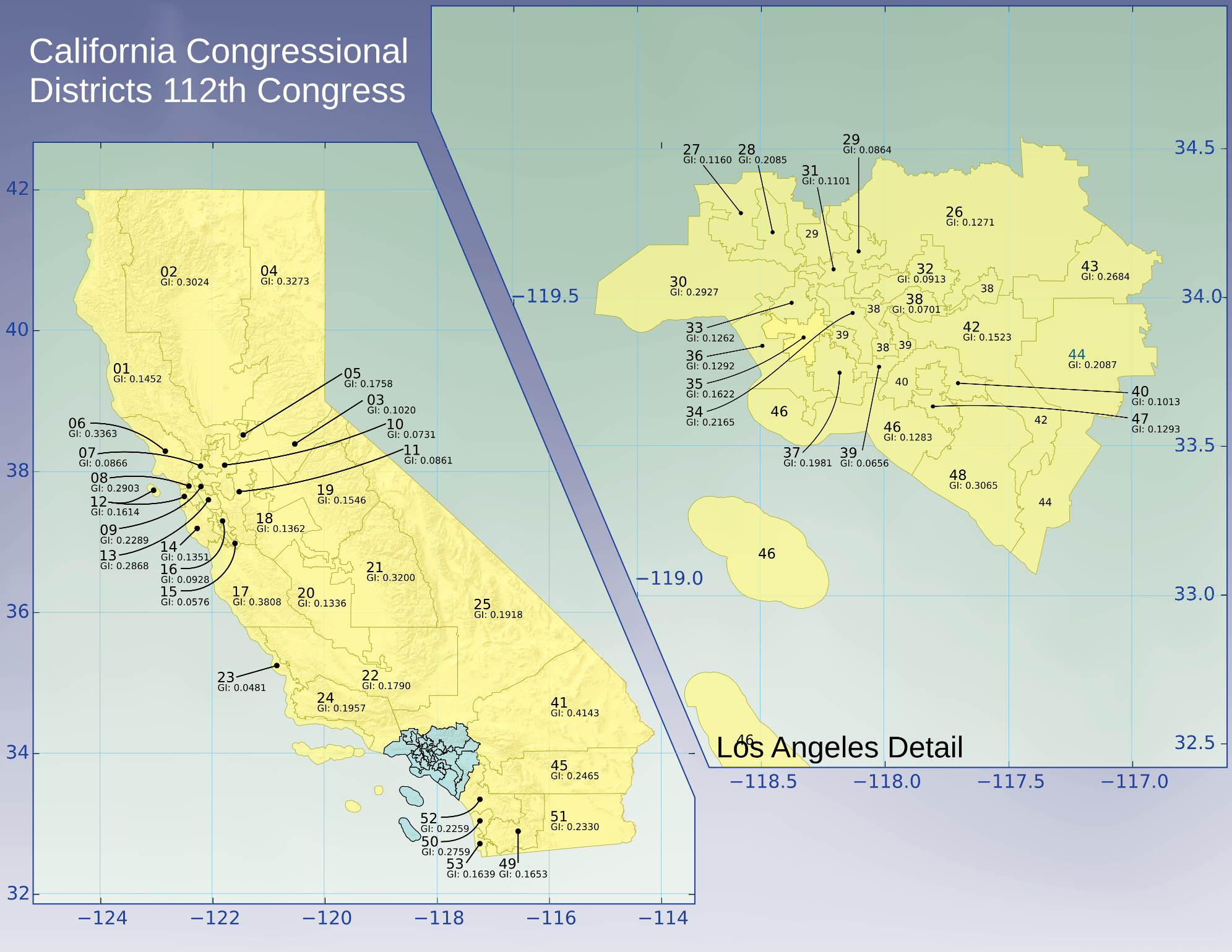
4. The redistricting plan drawn by the Califormia State legislature for the 112th Congress (2011-2013), the last one based on the 2000 Census.
The commission’s obligation is to establish districts which adhere to six criteria, in decreasing order of rank, population equality (“one man, one vote”), compliance with the Federal Voting Rights Act, geographical “continuity”, “integrity” and “compactness” and, if possible, the nesting of adjoining assembly districts into single senatorial districts. Criteria 3 through 5 interest us here as they are the “anti-gerrymandering” criteria. With one redistricting effort under its belt, how well did the commission do?
The last Congress apportioned according to 2000 Census data was the 112th, For California, that Congress also used the last redistricting plan drawn up by a California state legislature. California’s 53 congressional districts had an average Gerrymander Index of 0.182, ranging from a minimum of 0.048 (California Congressional District 23 – before 2013, a narrow ribbon running along the coast from Oxnard to the Monterey county line) to a maximum of 0.43 (California Congressional District 41), these calculated from the Census Bureau’s tl_2011_us_cd112 dataset for the 112th Congress.
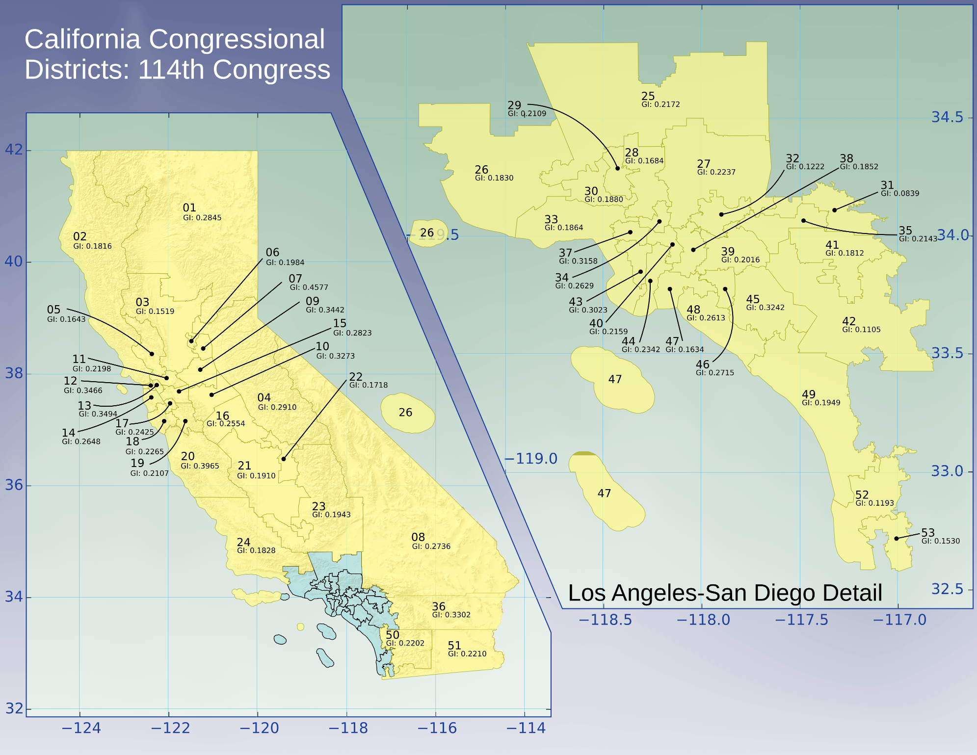
5. The first plan authored by California’s redistricting commission following Proposition 20. It is based on the 2010 Census.
For the 114th Congress, the state’s 53 congressional districts have an average Gerrymander Index of of 0.232, an up-tick of 0.05. The minimum is 0.084, belonging to California Congressional District 38, and the maximum is 0.458, belonging to California Congressional District 7.
A modest improvement, numerically, perhaps unremarkable in and of itself. However, after a decade of House elections where, perhaps, only one seat changed hands, the 2012 and 2014 California Congressional races offered a few more interesting runs. Four seats changed hands in 2012, compared to only one seat in 2002, the previous election that was held immediately after a redistricting. In fact, more seats changed hands in 2012 than in the previous five elections. In 2014, one seat changed hands, compared to no seats changing hands in 2004.
That said, a change of four or five seats in a delegation of fifty-three representatives is hardly a revolution. An up-tick; and one hopes not the last one.
Six years before California Proposition 11, Texas underwent a revolution of sorts. In 2002, the Republican Party won control of the Texas state legislature for the first time in 130 years. Its 2003 redistricting plan, promoted by Representative Tom DeLay (TX-22) and Governor Rick Perry, so appalled the fifty-two Democratic members, now in the minority, that they bolted the state to delay the plan’s passage, preventing a quorum in the state’s legislature. So began a protracted struggle that culminated, three years later, in The League of United Latin American Citizens v. Perry (2006). Those who dislike gerrymandering in any form find little comfort in this Supreme Court ruling. The Court found in a 7 – 2 decision that the 2003 Texas redistricting plan did not constitute political gerrymandering, nor was a State necessarily restricted to one redistricting effort per Census, but could redistrict anytime, as long as it is done at least once in ten years. Small comfort could be found in the Court’s narrow, 5 – 4 decision finding the newly drawn 23rd Congressional District discriminatory against the local Hispanic community.
The footprints of the 2003 redistricting plan may still be found in the Texas Congressional Districts for the 114th Congress. With a generally low average state Gerrymander Index of 0.1949, the 2nd, 18th, 29th, 33rd, and 35th districts all have indices below 0.1 and manifest bizarre shapes. All are urban districts, the first three in Houston, the fourth in the Dallas-Ft. Worth metroplex, and the last meandering from San Antonio to Austin in a manner reminiscent of North Carolina’s 12th district. We have been assured by the Supreme Court, however, that these are not partisan-motivated gerrymanders. So let us be assured.
To sum up, we think the Gerrymander Index is a succinct way to state a condition. It is a hard number, derived entirely from the geometry of a Congressional district. Essentially, Congressional districts which are more out of round, to wit: less like a circle, will give rise to lower Gerrymander Indices.
As a succinct way to state a condition of out-of-roundness, or lack of “compactness”, we’d like to see the Gerrymander Index become very popular. Alas, there are some barriers to this.
First, a Gerrymander Index is very, very sensitive to how one measures perimeters; perimeters that run along natural geological formations such as oceans, lakes, rivers or mountain ranges are subject to Richardson’s Paradox, to wit: the measure of lengths with ever more precise rulers does not converge to a particular limit distance, but grows without bounds, if the length exhibits a fractal dimension, which, alas, many natural boundaries do. As a consequence one cannot quote Gerrymander Indices in isolation, but should be prepared to state the geometry from which the index was computed. Saying that the 9th New York Congressional District has a Gerrymander Index of 0.296 without saying from which data set the number was computed is essentially saying nothing at all.
Second, stemming from the first, there are no “authoritative” sources of boundary geometry. We have been using geometry provided by the Census Bureau, but the Census Bureau goes to pains to indicate that their data are for making display maps; that the data are altered to render boundaries nicely at certain resolutions. We stick with this dataset because its data have been messed with in a consistent way, so there is reason to hope that one can compare Gerrymander Indices among Congressional Districts so long as we stick with the same Census Bureau dataset. That may be fine for a “blue sky” kind of political post, but a serious discussion needs to be grounded in authoritative data. Recognizing authoritative data in these politically polarized times might be tricky.
These limitations, while substantial, are not fatal. What is needed by citizens when conversing with their elected representatives is a concise way of stating how a public boundary may be malformed. If the need for that mechanism is felt strongly enough, these limitations can be overcome.
We hope, by incorporating the Gerrymander Index into the National Discourse, that useful “Races to the Bottom” might occur in places where gerrymandering is epidemic. When one political party beats down the High-GI numbers arising from the previous party in power, it wins bragging rights. And when the political pendulum sweeps the other party back in, the new State legislature or Districting Commission will think twice before redrawing Congressional districts in a gerrymandered way, pushing that dreaded GI number back up again.
The real winners will be citizens, who suddenly find themselves in neither packed, one party district ghettos, their political reach reduced by their concentration, nor cracked out into different districts, where they are perpetual minorities. Instead they may find themselves in rather somewhat rounded districts, containing something like full political spectra. To advance their political ideals, they may even have rediscover the art of political discourse, as the artifice of gerrymandering fades from the political scene. Representatives to Congress may even have to re-acquire the knack of representing politically diverse districts again. One could hope.
i All Gerrymander Index citations in this post were calculated from boundary data from the shape file data set, tl_2014_us_cd114, available from the Census Bureau, Department of Commerce
Fascinating series, Thanks.
But I think a better way to define the index would be to compute the inverse of the index you use. That would give Indiana a GI of 2.2936, IN-1 1.7825, and IN-8 4.6083. NC, on the other hand, would have a GI of 8.5470, NC-12, 40.1606. This gives us an (arbitrary) subjective definition: if a district has a GI > 5, or 6, it appears to be Gerrymandered. This is actually more intuitive: the larger the number, the greater the level of Gerrymandering.
You could argue that it’s arbitrary, but all scales are arbitrary. Farenheit used the freezing point of the Atlantic for 0 and his personal body temperature for 100 – and he was running a fever that day. Celcius is similarly arbitrary, but more “scientific,” he used the freezing and boiling points of pure water at sea level for 0 and 100.
Even the meter is an arbitrary number, according to Wikipedia (https://en.wikipedia.org/wiki/Metre), “The metre was originally defined in 1793 as one ten-millionth of the distance from the equator to the North Pole. In 1889, it was redefined in terms of a prototype metre bar (the actual bar used was subsequently changed twice). In 1960, the metre was redefined in terms of a certain number of wavelengths of a certain emission line of krypton-86. In 1983, the current definition was adopted. In 1959, the imperial inch was re-defined as 0.0254 metres (2.54 centimetres or 25.4 millimetres). One metre is about 3 3⁄8 inches longer than a yard, i.e. about 39 3⁄8 inches.”
I suppose if the American Revolution had begun in 1794, not 1776 (or we had lost) we would be using the metric system.